Hello, people…! In this post, I will talk about one of the fastest single source shortest path algorithms, which is, the Dijkstra’s Algorithm. The Dijkstra’s Algorithm works on a weighted graph with non-negative edge weights and gives a Shortest Path Tree. It is a greedy algorithm, which sort of mimics the working of breadth first search and depth first search.
The Dijkstra’s Algorithm starts with a source vertex ‘s‘ and explores the whole graph. We will use the following elements to compute the shortest paths –
- Priority Queue Q.
- An array D, which keeps the record of the total distance from starting vertex s to all other vertices.
Just like the other graph search algorithms, Dijkstra’s Algorithm is best understood by listing out the algorithm in a step-by-step process –
- The Initialisation –
- D[s], which is the shortest distance to s is set to 0. The distance from the source to itself is 0.
- For all the other vertices V, D[V] is set to infinity as we do not have a path yet to them, so we simply say that the distance to them is infinity.
- The Priority Queue Q, is constructed which is initially holds all the vertices of the graph. Each vertex V will have the priority D[V].
- The Algorithm –
- Now, pick up the minimum priority (D[V]) element from Q (which removes it from Q). For the first time, this operation would obviously give s.
- For all the vertices, v, adjacent to s, i.e., check if the edge from s → v gives a shorter path. This is done by checking the following condition –
if, D[s] + (weight of edge s → v) < D[v], we found a new shorter route, so update D[v]
D[v] = D[s] + (weight of edge s → v) - Now pick the next minimum priority element from Q, and repeat the process until there are no elements left in Q.
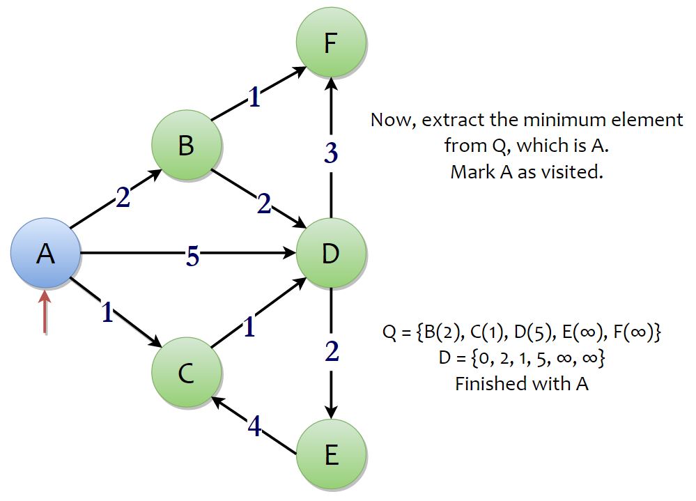
Let us understand this with the help of an example. Consider the graph below –
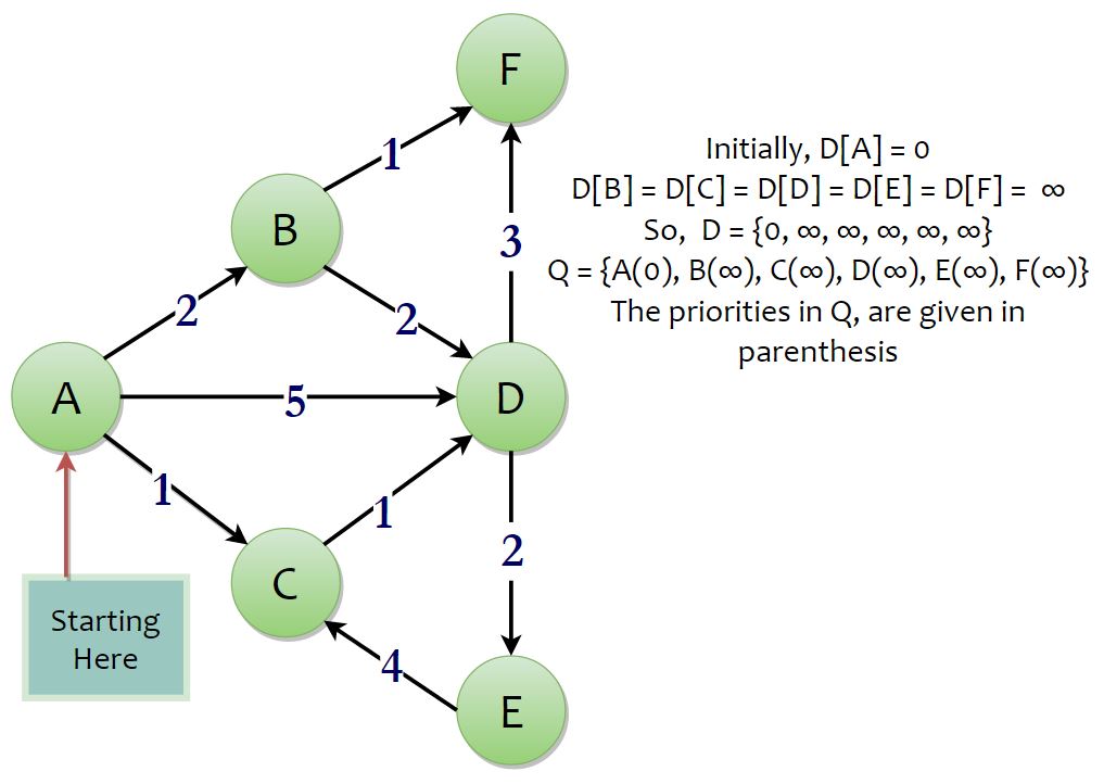 Firstly, initialize your components, the shortest distances array D, the priority queue Q. The distance from the source to itself is zero. So, D[s] = 0, and the rest of the array is ∞. The set of vertices v is inserted into the priority queue Q, with a priority D[v]. Now, we start our algorithm by extracting the minimum element from the priority queue.
The minimum element in the priority queue will definitely be s (which is A here). Look at all the adjacent vertices of A. Vertices B, C, D are adjacent to A. We can go to B travelling the edge of weight 2, to C travelling an edge of weight 1, to D travelling an edge of weight 5. The values of D[B], D[C], D[D] are ∞ . We have found a new way of reaching them in 2, 1, 5 units respectively, which is less than ∞, hence a shorter path. This is what the if-condition mentioned above does. So, we update the values of D[B], D[C], D[D] and the priorities of B, C, D, in the priority queue. With this, we have finished processing the vertex A.
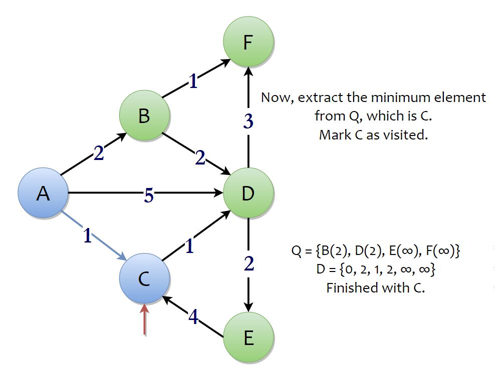
Now, the process continues to its next iteration and we extract the minimum element from the priority queue. The minimum element would be vertex C which would be having a priority of 1. Now, look at all the adjacent vertices to C. There’s vertex D. From C, it would take 1 unit of distance to reach D. But to reach C in prior, you need 1 more unit of distance. So, if you go to D, via C, the total distance would be 2 units, which is less than the current value of shortest distance discovered to D, D[D] = 5. So, we reduce the value of D[D] to 2. This reduction is also called as “Relaxation“. With that, we’re done with vertex C.
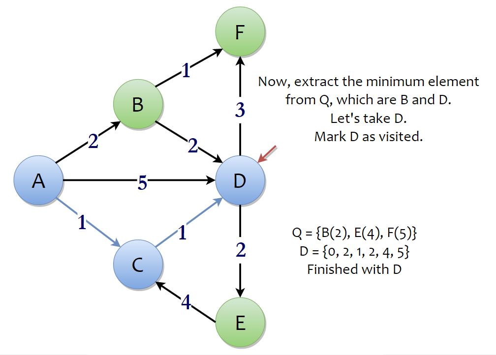
Now, the process continues to its next iteration and we extract the minimum element from the priority queue. Now, there are two minimum elements, B and D. You can go for anyone. We will go for vertex D. From D, you can go to E and F, with a total distance of 2 + 2 {D[D] + (weight of D → E)}, and 2 + 3. Which is less than ∞, so D[E] becomes 4 and D[F] becomes 5. We’re done with vertex D.
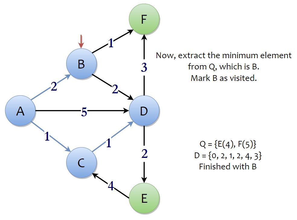
Now, the process continues to its next iteration and we extract the minimum element from the priority queue. The minimum element in the priority queue is vertex B. From vertex B, you can reach F in 2 + 1 units of distance, which is less than the current value of D[F], 5. So, we relax D(F) to 3. From vertex B, you can reach vertex D in 2 + 2 units of distance, which is more than the current value of D(D), 2. This route is not considered as it is clearly proven to be a longer route. With that, we’re done with vertex B.
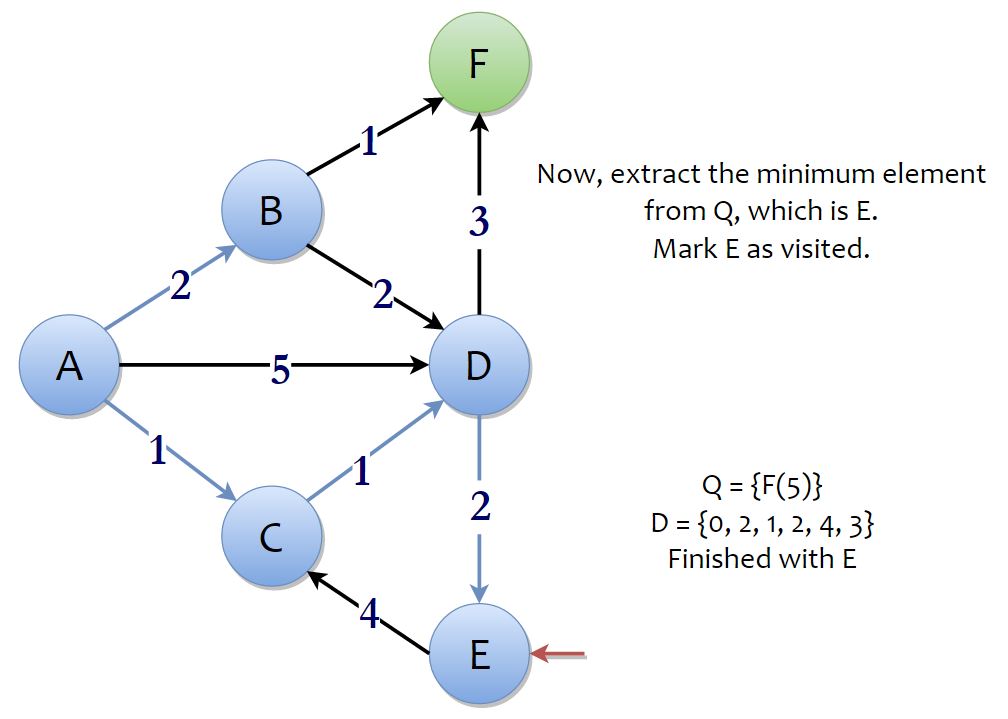 Now, the process continues to its next iteration and we extract the minimum element from the priority queue. The minimum element in the priority queue is vertex E. From vertex E, you can reach vertex C in 4 + 4 units of distance, which is more than the current value of D(C), 1. This route is not considered as it is clearly proven to be a longer route. With that, we’re done with vertex E.
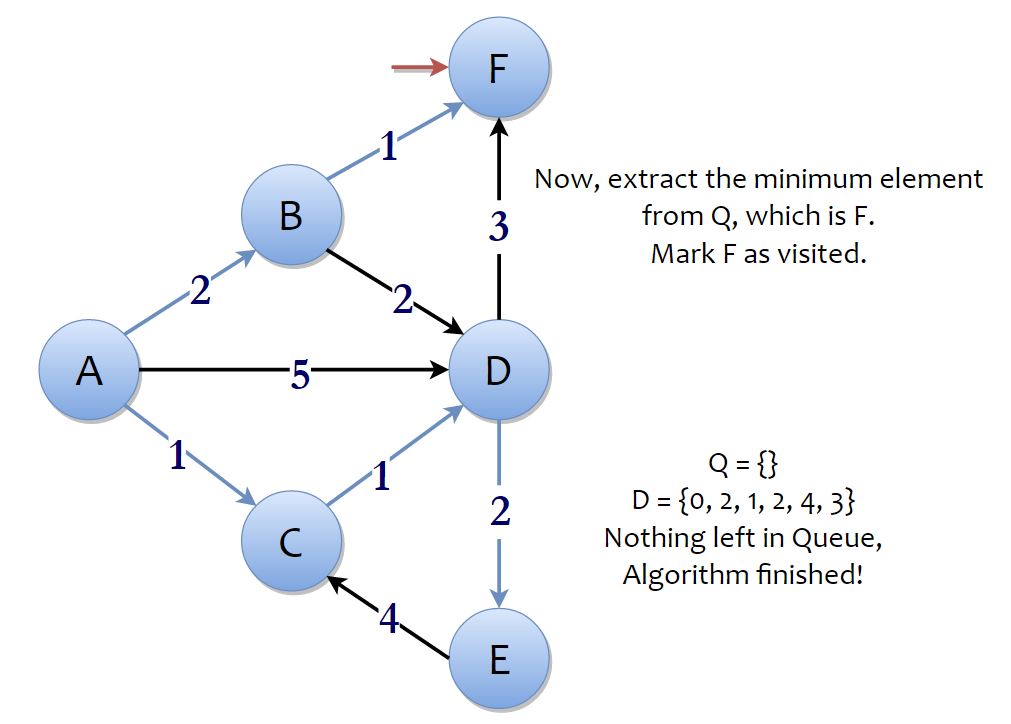 Now, the process continues to its next iteration and we extract the minimum element from the priority queue. The minimum element in the priority queue is vertex F. You cannot go to any other vertex from vertex F, so, we’re done with vertex F.
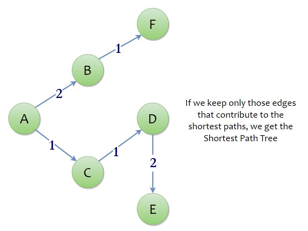 With the removal of vertex F, our priority queue becomes empty. So, our algorithm is done…! You can simply return the array D to output the shortest paths.
Having got an idea about the overall working of the Dijkstra’s Algorithm, it’s time to look at the pseudo-code –
dijsktra(G, S)
D(S) = 0
Q = G(V)
while (Q != NULL)
u = extractMin(Q)
for all V in adjacencyList[u]
if (D(u) + weight of edge &lt; D(V))
D(V) = D(u) + weight of edge
decreasePriority(Q, V)
In the pseudo-code, G is the input graph and S is the starting vertex. I hope you understand the pseudo-code. If you don’t, feel free to comment your doubts. Now, before we code Dijkstra’s Algorithm, we must first prepare a tool, which is the Priority Queue.
The Priority Queue
The Priority Queue is implemented by a number of data structures such as the Binary Heap, Binomial Heap, Fibonacci Heap, etc. The priority queue in my code is implemented by a simple Binary Min Heap. If you are not aware about the Binary Heap, you can refer to my post on Binary Heaps. Now the functionalities that we need from our priority queue are –
- Build Heap – O(|V|) procedure to construct the heap data structure.
- Extract Min – O(log |V|) procedure, where we return the top-most element from the Binary Heap and delete it. Finally, we make the necessary changes to the data structure.
- Decrease Key – We decrease the priority of an element in the priority queue when we find a shorter path, as known as Relaxation.
If you know the working of the Binary Heap you can code the Priority Queue in about 1-2 hours. Alternatively, you can use C++ STL’s priority queue instead. But you don’t have a “decrease key” method there. So, if you want to use C++ STL’s priority queue, instead of removing elements, you can re-insert the same element with the lowered priority value.
Simple O(|V|2) Implementation
If you choose to implement priority queue simply by using an array, you can achieve the minimum operation in O(N) time. This will give your algorithm a total runtime complexity of O(|V|2). It is the simplest version of Dijkstra’s algorithm. This is the version you are supposed to use if you quickly want to code the Dijkstra’s algorithm for competitive programming, without having to use any fancy data structures. Take a look at the pseudocode again and try to code the algorithm using an array as the priority queue. You can use my code below as a reference –
Faster O(|E| log |V|) implementation
You can use a binary heap as a priority queue. But remember that to perform the decrease-key operation, you’ll need to know the index of the vertex inside the binary heap array. For that, you’ll need an additional array to store a vertex’s index. Each time any change is made in the binary heap array, corresponding changes must be made in the auxiliary array. Personally, I don’t like this version but I’ll put my code below so that you can use it as a reference.
If you want to do the same thing in C++, you can use a priority queue to reduce a lot. The tweak here is that because you cannot remove a certain vertex from a C++ STL priority queue, we can re-insert it with the new lower priority. This will increase the memory consumption but trust me, its worth it. I have put the codes for both versions below.
The complexity of the above codes is actually O(|V| + |E|) ✗ O(log |V|), which finally makes it O(|E| log |V|). Dijkstra’s Algorithm can be improved by using a Fibonacci Heap as a Priority Queue, where the complexity reduces to O(|V| log |V| + |E|). Because the Fibonacci Heap takes constant time for Decrease Key operation. But the Fibonacci Heap is an incredibly advanced and difficult data structure to code. We’ll talk about that implementation later.
This is the Dijkstra’s Algorithm. If you don’t understand anything or if you have any doubts. Feel free to comment them. I really hope my post has helped you in understanding the Dijkstra’s Algorithm. If it did, let me know by commenting. I tried my best to keep it as simple as possible. Keep practising and… Happy Coding…! 🙂

31 thoughts on “Dijkstra’s Algorithm”
sir, i’m just a beginner in data structure. my doubt will seem to be silly but i hope u will reply soon as this doubt is frustating me. The priority queue created has all distances initialised as infinity except for the start vertex. how can we the implement heapify finction in which different distances are to be compared.
I cant find where the distances have been changed?pls help…
I didn’t understand your question fully. What do you exactly mean by “in which different distances are to be compared”? The code for heapify function I used is given in the post. Try to go through that method and see if it answers your question.
Great explaination … simple and straight …
I think if you provide some example atleast one below the code this will definitely worked more to understand otherwise superb
awesome! helped me a lot thankyou. Im trying to implement this by fibonacci heap.Can you please help
Fibonacci heap is pretty complex. Never implemented it myself. 😛
Very well explained. Thank you
I am not able to understand the use of hashTable[] properly.
Yes I get that it is for storing the location of vertex i, but the thing which is confusing me is, in the starting at the time of scanning the nodes, the new node’s ‘label’ is the ‘value’ of the hashTable[] while ‘i’ is the ‘key’ and in the heapify procedure, the ‘label’ is being used as the ‘key’ while ‘i’ to be the ‘value’.
Please give a bit detailed explanation for this plus what is the real necessity of taking this hashTable[].
One more thing, are you assuming ‘labels’ to be same as the ‘index’ number at which the node is being stored initially in minHeap[]..i.e from 1 to n only ?
If yes, then what if the labeling is not done in this particular order… what will happen then ?
I completely understand the use of hashTable[] after thinking precisely on its working so you don’t need to explain that part now 😀
But still there is a thing which is a bit problematic to me, i.e If the vertices scanned do not range from [1…vertices] (and have value larger than ‘vertices’) , in that case would we not be able to store the location of the vertex in hashTable[]..?
In my opinion we won’t be able to do that.
Please correct me if I am wrong, and if if not then what would be the solution of that case..?
And Very Thank You for the post 😀 😀
Surely it is the tough algorithm and takes time in the starting to understand each section, but your explanation made it really very helpful to get and code it properly.
Thanks again 🙂
Is there any disadvantage if I implement Dijkstra’s Algorithm using std::priority_queue ??
Sorry for the late reply…. Well firstly, even when u have an STL priority queue, you will need a hash table to map the vertices to their indices on the priority queue and secondly, we are using an operation called DecreaseKey() where we lower the priority of an element in the priority queue, and then bubble it up to ensure the structure stays as a heap… Now we don’t have any specific STL function to do that bubbling up for you… So you would have to implement that one function DecreaseKey() by yourself and the rest is taken care by STL… And the complexities stay same as the priority queue in STL is internally a vector or a dequeue which performs similar to an array… 🙂
I did not change the priority of element I just kept on inserting them. Since we take minimum priority element each time we will get correct priority of an element. Although space complexity increases a bit in this approach because of multiple copies of same element, I think it will give correct answer.
Here is my implementation :- http://ideone.com/ugfGvV
Well, it does seem to work, but I’m still skeptical about that approach… I’ll let you know if I find any counter examples for your approach… But I do suggest you to try the standard algorithm too 🙂
i need input values for abouvegraph example not input format…pls give
The input values are in the file whose link is given in my reply…
pls can anyone give input for which that code will work
It’s better if u give input for above example
The input format is… The first line has 2 integers N and E, the number of nodes and the edges in the graph. This is followed by E number of lines, each consisting of 3 integers, U, V, W… This represents an edge between U and V of weight W. This followed by the last line of the input which is a single integer which is the starting vertex of the algorithm.
This is the input file I used to test my code for large input. It is a bi-directional graph where each edge has different weight. The vertices in the input are 1-indexed… 🙂
Pls give code till tomorrow
Pls give code for modified dijkstra’s Algorithm …( one of its application telephone network)
http://www.csl.mtu.edu/cs2321/www/newLectures/30_More_Dijkstra.htm
Sure, Siya…. 🙂 … I’ll write the posts in a couple of weeks 🙂
why this code give Segmentation fault (core dumped)
My end semester exams are going on..! So it is a difficult for me to give the code any soon.. btw… Can you comment the input for which my code gave you segmentation fault..?
Can you give input for which that code will w
Can you give input for which that code will work
It’s better if u give input for above example
Helped me understand it much better….Thank you
I’m glad I could help you Jenil 🙂
this is a much shorter version of dijkstra using stl set, what do u think??
http://ideone.com/yNE4Au
Amazing Explanation!
Could you also post some links to spoj or codechef questions regarding the above algorithm it would be extremely useful 🙂
Sure..! Your suggestion is great..! I’ll see what I can do… 🙂
Hey there!
Awsome code but I have a small question:
How can I track a particular path from the first node to a desired node?
Hi @Perez..! It was silly of me that I didn’t include that in a Single Source Shortest Path Algorithm…! 😛 … Thanks to remind me..! 🙂 … I have updated the code to print the shortest path also. In order to get the shortest path, we need more information… We need to know the parent node of each node in the shortest path.. That is… The vertex via which we had to come, to get the shortest path. To store this additional information, I convert the shortestDistances array to an array of pairs. The elements of the pair store –
Then I have made slight changes to the algorithm to get the parents. The changes are in lines 188, 193, 231. They don’t affect the performance of the algorithm. Once you get the information about the parents… To compute the shortest path from E → A, all you have to do is to recursively look at each vertex’s parent. That is exactly what PrintShortestPath() function does. Just give it a little thought, I’m sure you’ll understand it..! I will update my post to include the required explanation in a few days… Feel free to ask if you have any more doubts..! 😀