Every programmer needs a suitable data structure to compute some complex function or to do a time-taking task quickly. In this post, I will explain the Binary Indexed Tree (BIT) data structure also known as the Fenwick Tree in post-soviet countries. This data structure is very easy to code in competitions. So, a programmer who knows BIT will have a massive edge over others. But the problem with BIT is that it is NOT easy to understand! A beginner may go nuts in trying to understand the working of a Binary Indexed Tree. I will explain this data structure step-by-step using as many images, tables and examples as I can.
Binary Indexed Tree becomes handy in manipulating Cumulative Frequency Tables. Now, I assume you know what Frequency and Cumulative Frequency is! Now, consider we have 12 objects with us of the respective frequencies –
| Item No. | Frequency | Cumulative Frequency |
|---|---|---|
| 1 | 4 | 4 |
| 2 | 2 | 6 |
| 3 | 7 | 13 |
| 4 | 5 | 18 |
| 5 | 1 | 19 |
| 6 | 3 | 22 |
| 7 | 6 | 28 |
| 8 | 4 | 32 |
| 9 | 6 | 38 |
| 10 | 6 | 44 |
| 11 | 3 | 47 |
| 12 | 3 | 50 |
Now, if we were to increase the quantity of Item 5 by 1. We would have to change the whole table. The change would be like,
| Item No. | Frequency | Cumulative Frequency |
|---|---|---|
| 1 | 4 | 4 |
| 2 | 2 | 6 |
| 3 | 7 | 13 |
| 4 | 5 | 18 |
| 5 | 1 + 1 | 19 + 1 |
| 6 | 3 | 22 + 1 |
| 7 | 6 | 28 + 1 |
| 8 | 4 | 32 + 1 |
| 9 | 6 | 38 + 1 |
| 10 | 6 | 44 + 1 |
| 11 | 3 | 47 + 1 |
| 12 | 3 | 50 + 1 |
If we were to code this manipulation using an array of integers, the implementation would go like,
| Array Element | Element Value |
|---|---|
| arr[0] | 4 |
| arr[1] | 6 |
| arr[2] | 13 |
| arr[3] | 18 |
| arr[4] | 19 + 1 |
| arr[5] | 22 + 1 |
| arr[6] | 28 + 1 |
| arr[7] | 32 + 1 |
| arr[8] | 38 + 1 |
| arr[9] | 44 + 1 |
| arr[10] | 47 + 1 |
| arr[11] | 50 + 1 |
Clearly, implementing the simple increment would cost O(n). This is because in Cumulative Frequency, every element holds the “prefix-sum” of the elements, i.e., the sum of elements till that index. Now what if we hold only partial sums? Say, there are three variables that hold the partial sums and the final sums can be evaluated by summing up the partial sum. Now, the question arises is, “How does this help the increment manipulation?”. This is explained by the following diagram.
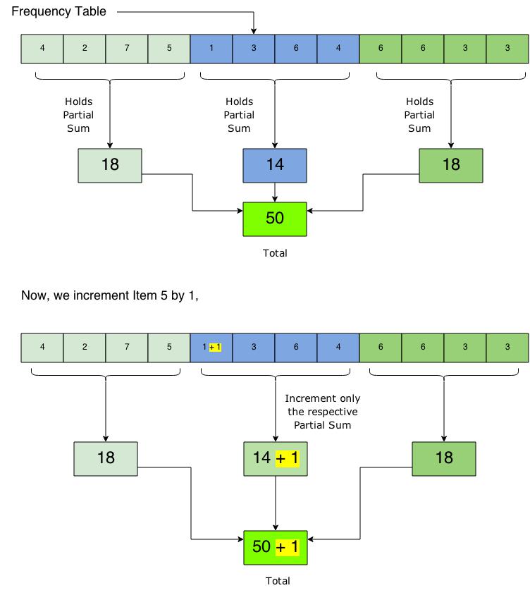
So, we can see how by using the Partial Sum Technique, we managed to decrease the number of operations to perform. This is the raw underlying idea of the Binary Indexed Tree. But the Binary Indexed Tree uses this partial sum technique far more efficiently and quite amazingly actually! The BIT is constructed on the principle that “all numbers can be represented as the sums of powers of 2”. This is more or less similar to the principle behind the binary numbers. Now the working of the BIT is that, at indices
of the values of powers of 2, they contain the total sum of the frequencies till that index. Which means if we have an element of an array, arr[7], it will have the sum of elements from arr[0] to arr[7] (including the value of arr[7], i.e, frequency of the 8th element). Thats ok! But what will the other elements contain…?! The Partial Sums…! I make this clear with the help of my next sketch where I show a simple Binary Search Tree (BST) where the nodes have the values of the frequencies and the nodes are constructed in such a way that the value of the “index” is taken into consideration while constructing the BST but the nodes hold the frequencies as the values. Then I will give a super simple step-by-step explanation.
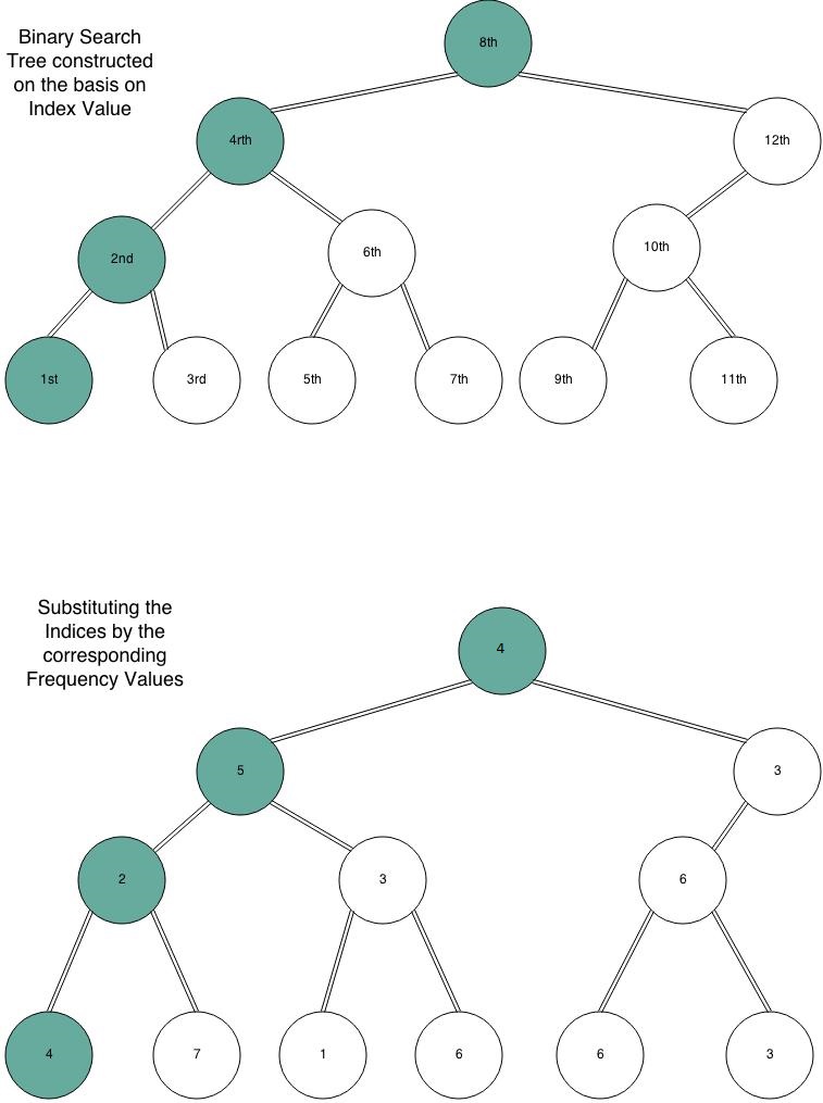
We all know that the Binary Search Tree is such that the left-subtree holds all the values less than the current node. Now, the Binary Indexed tree is such that, the current node holds the sum of all values in it’s left-subtree + the value of the current node. For example, in the first tree in the above image,
Value of Node 10 = Value of Node 9 + Value of Node 10
Value of Node 12 = Values of Node 12 + Value of Node 10 (= Value of Node 9 + Value of Node 10…!)
Similarly,
Value of Node 4 = Values of Node 4 + Value of Node 3 + Value of Node 2 (= Value of Node 2 + Value of Node 1…!)
So, now we see that the Node 4 will be the sum of Nodes 1 to 4, similar is the case with all the nodes that are powers of 2. These nodes are somewhat special, as they contain the “prefix-sum”. Hence, I marked them in my previous image. Now we will apply the concept to our second tree in the above image.

Wait…! What…?! The “array” is the “tree”…?! Yes…! The array we obtained is called the Binary Indexed Tree. For whatever applications a BIT is used for, it is used as this array. Pretty cool, uh…! So, this means you don’t have to get messed up creating structures, pointers and doing tree travels! All you’ll need is this simple array. Now, before we get into the coding part of the BIT lets observe this BIT “array” a little more closely so that we can understand it more clearly. Again, I use an image because we all know, “A picture speaks more than a thousand words!”.
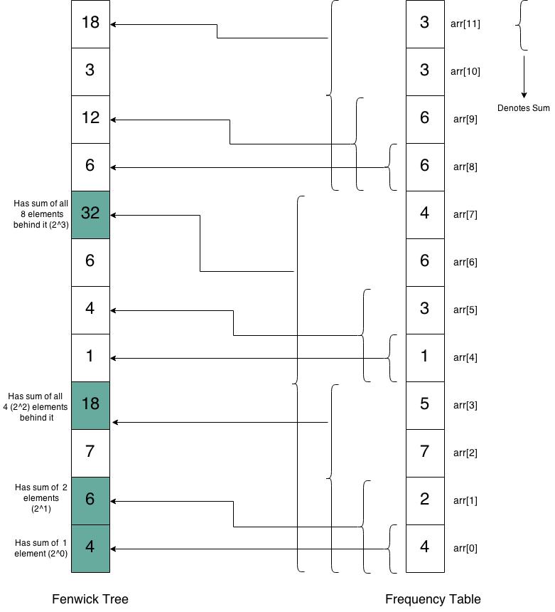
The picture clearly shows how the Fenwick Tree (or BIT) stores the partial sums and that at indices of powers of two it will have the complete sum of all the elements behind it. What really allows the Fenwick Tree to have this feature is the very structure of the Binary Search Tree (BST). In a BST, the nodes with index in powers of two lie at the left-most part of the tree (recall our very first tree of the first image), now, we know for a Binary Indexed Tree, the value of a node is the sum of the components of the left-subtree + the value that is supposed to be in that node. But what will the left-subtree of a Binary Search Tree have?… “Some” elements surely less than it. Now, what will the left-subtree of the left-most wing of a tree have? “All” the elements surely less than it. If you ponder on this statement for a while you will understand why the indices of the powers of 2 have the whole “prefix-sum”. Now I will depict you the effect of increment of an Item in the Binary Indexed Tree, for this I use the tree representation once again.
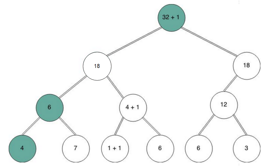
As we can clearly see, in a worst case scenario, such as the above, we’d have to update all the nodes beginning from the lowest level and go up till the root node. So, in a worst case scenario, we’d have to update the “height of the tree” number of nodes, which is log n as we know it. So, the increment operation here costs only O(log n), which is very fast! Recall that our brute force or the naive approach costed us O(n), so now we know how using BIT speeds up the manipulation. But how do we do this in an array? For a given frequency table, how do we construct the BIT? We will see this coding part now, which is also difficult to understand but easy to implement.
For a given frequency array freq[] of size ‘n’, create another array bit[] of size ‘n’ and initialize bit[] to zero. Now, run a loop where we take every element of freq[] one-by-one and put it into bit[]. What actually are we doing is that we are doing the increment operation over and over again. Look over the code closely –
You might feel uncomfortable with the “j = j + (j & (-j))” thing, for now, forget that, we’ll come back to it in a minute. Look what is logically happening in the code. Being able to read raw code is a gift, if you can, you’re awesome! Be proud of it! For those who can’t, here is what happening. Listen carefully!… First we take the collection of items to be empty, so, all items have zero frequency. Then, we take the first item, it’s frequency is 4, so we “increment” the frequency of that item from 0 → 4. Now, recall the picture of the effect of increment in Fenwick Trees. I drew a Binary Search Tree and incremented the leaf node and up till the root by 1. Here, we will increment by 4, all the corresponding log n nodes. For better understanding watch the picture below closely –
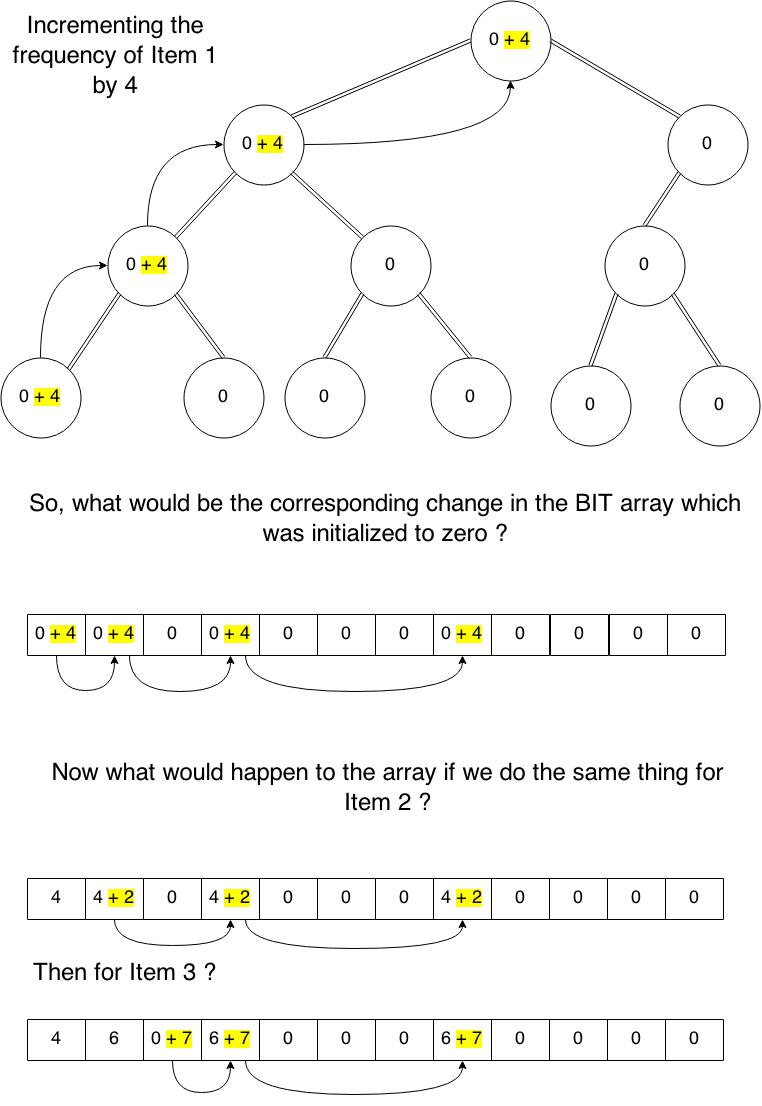
It is clear from the explanation how the Fenwick Tree gets going. But how does one traverse so strangely, I mean, the first Item we had to go like, 1 → 2 → 4 → 8, then for the next Item we had to go like, 2 → 4 → 8, and then like 3 → 4 → 8…! How does one put it in a code? This is exactly what “j = j + (j & (-j))” does! It takes you to the next location where you are to increment the value. It is a standard expression for traversing a Fenwick Tree. If you are really eager to understand the logic behind the standard expression, you have to read this wonderful blog by Devendra Agarwal. It was where I was able to start my BIT journey. Lastly, I will just show you an output of the same above code but with little modification so that it prints the values of variables and BIT array step-by-step.
If you have understood till here, you will be able to understand the output without breaking a sweat. I will conclude this post here. It has become too large already, and I guess my reader’s would also like a break. Thanks a lot for being so patient with me! If you really are eager to do some questions on this topic, go for Insertion Sort Advanced Analysis of HackerRank. I enjoyed solving that question, and I hope you will too! Feel free to comment your doubts..! Keep practising…! Happy Coding…! 🙂

33 thoughts on “Binary Indexed Tree (or) Fenwick Tree”
The code section is not showing on my browser. I tried on chrome and mozilla. Can you kindly look at the issue. Thanks.
Fixed it! Thanks for pointing it out 🙂
value of node 12=value of node 12+11+10+9
but it is given that
value of node 12=value of node 12+10+9
That’s a nicely made answer to a chlenlaging question
Thank you! 🙂
I think the admin of this website is acxtually working hard for his site, because here every stuff is quality based
data.
I do… Thanks a lot 😀
It’s remarkable to visit this website and reading the views of
all friends about this post, whilpe I am also eager
of getting knowledge.
Thank you 🙂
U r just amazing.Tried other articles but couldn’t understand anything.Diagrams make it so cool and that uncomfortable part of code .
Thank you..! 😀
Dude, You made my day. I read this from approx 7-8 tutorials but didnt fully understand ANY of them, But your blog is the lifesaver for me. I hope you keep on writing about RMQ. We really need your simple yet fantastic explaination.
Thanks a lot..! Glad I could be of help… Yeah, I’ll keep RMQ in mind… 😀
You are awesome Vamsi. I started studying BIT from topcoder tutorial. I read that several times but didn’t understand it. Then from geeks for geeks I got the link of your tutorial. Believe me I read your tutorial only once and understood it. Great work! If possible please write tutorials on :
1.) Light Heavy decomposition.
2.) Treaps.
3.) RMQ using sparse matrix.
4.) LCA and RMQ conversion.
Whoa…! Sounds great.. 😛 … I’ll try… 😀
Is there any proper way for constructing the BST from the indexes because constructing a BST with the same indexes but different root may give a varied result.
Umm… I took the BST to explain Binary Indexed Tree…. It could have been a normal Binary Tree too…. I’ll add the BST to my to-do list… Then you can see how we can construct a BST… 🙂
Very nice tutorials sir. wonderful explanations with diagrams 🙂
Thanks a lot…!! 😀
Very nice tutorial…can you please write a blog for range update with detailed explanation ?
Sure…! I’ll see what I can do Ajit… 😀
If my understanding is correct, In your tree diagram, when you update arr[4] to 1+1. The node with value 18, shouldn’t become 18+1. As the index of that node is lower that the index where update happened.
Correct me, if I’m wrong.
Yes, you are absolutely right @Prankur..! I violated the basic rule – “current node holds the sum of all values in its left-subtree + the value of the current node”. So any updations in the right subtree shouldn’t affect the parent node… I have updated the diagram… Thanks a lot for correcting me…! 😀
Nice !!!
Thank you…! 🙂
Much better and simple than any tutorial
Thanks a lot Ankit..! 🙂
Thanks! It was of help!
Happy to help Dhananjay…! 🙂
This Tutorial was far better than the TOPCODER and .geeksforgeeks …:D loved the explanation!!!!
Thank you Gohan…! 🙂 … I am happy that I could help you….! 😀